Test Case 1 Post Processing Information
Data Submittal Forms
HLPW6 is utilizing Github for submission of data files. The HLPW6 TC1 submission repo provides details on the files desired for submission. Some details on flow and surface visualization are provided below. Participants are requested to create a “fork” of the repository and generate merge requests for data upload. A detailed description of this methodology is provided here.
Post Processing: Upper Surface Streamlines and Skin Friction Coefficient (Cf) Contours
Postprocessing: Upper Surface Streamlines and Skin Friction Coefficient (Cf) Contours A major set of desired inputs from the CFD are computed surface streamlines, for qualitative comparison between datasets. This is particularly important for ascertaining the agreement/disagreement with regions of separation and other flow features of interest. Below is an example surface streamline plot, showing typical areas of interest for HLPW-4. There are many methods available for obtaining postprocessed surface streamline patterns; at this time, participants are encouraged to make use of the best tools at their disposal.
Contours of surface skin friction coefficient are also very useful to plot (see second figure immediately below). We are requesting plots of skin friction magnitude (tau_w/freestream dynamic pressure), not plots of its x-component. Note that the definition of tau_w is standard: see, e.g., Wall Shear Stress Definition, with the derivative of the flow velocity parallel to the wall used in the equation. Within the Scale Resolving TFG, both temporally averaged and instantaneous skin friction plots are requested.
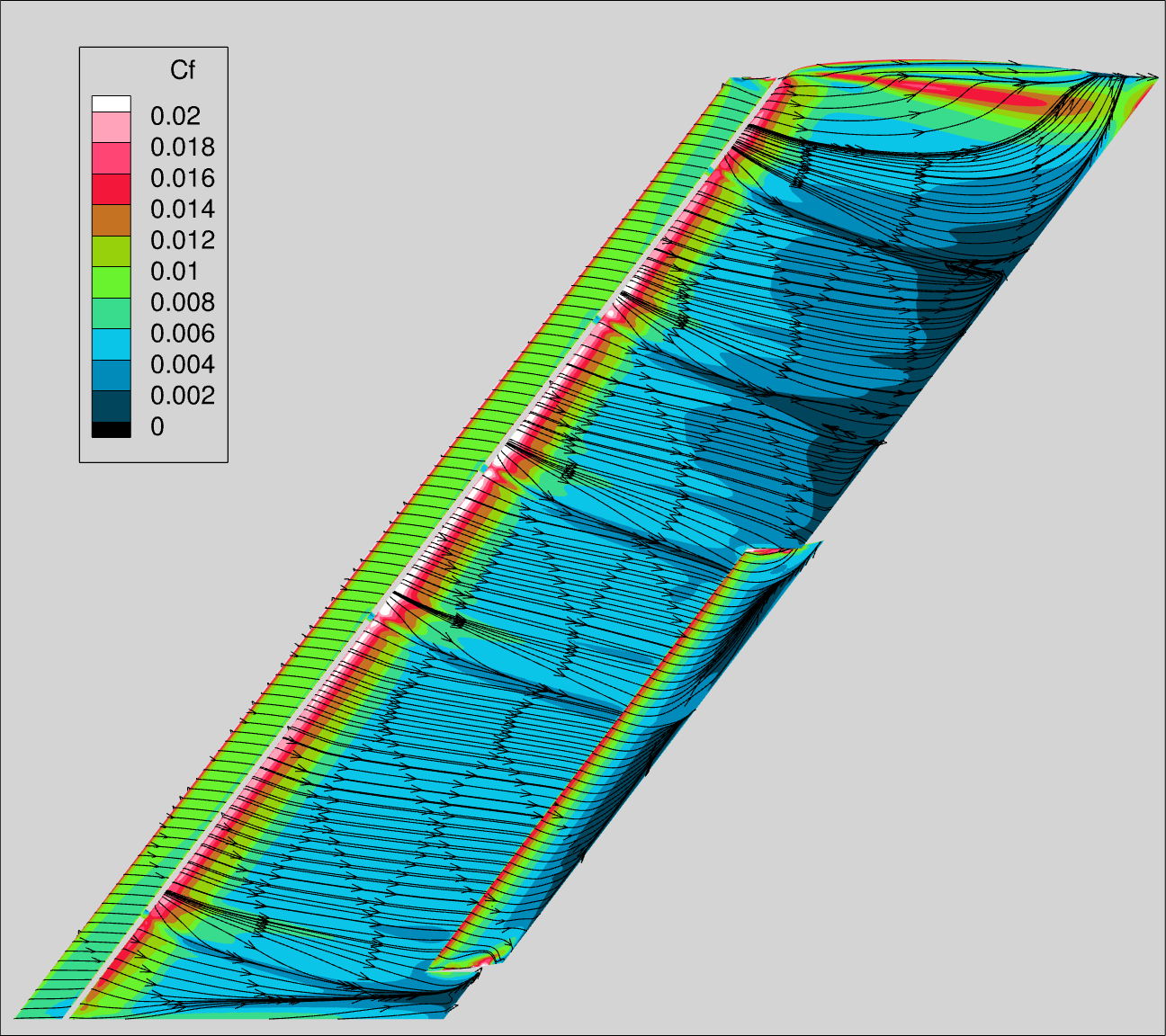
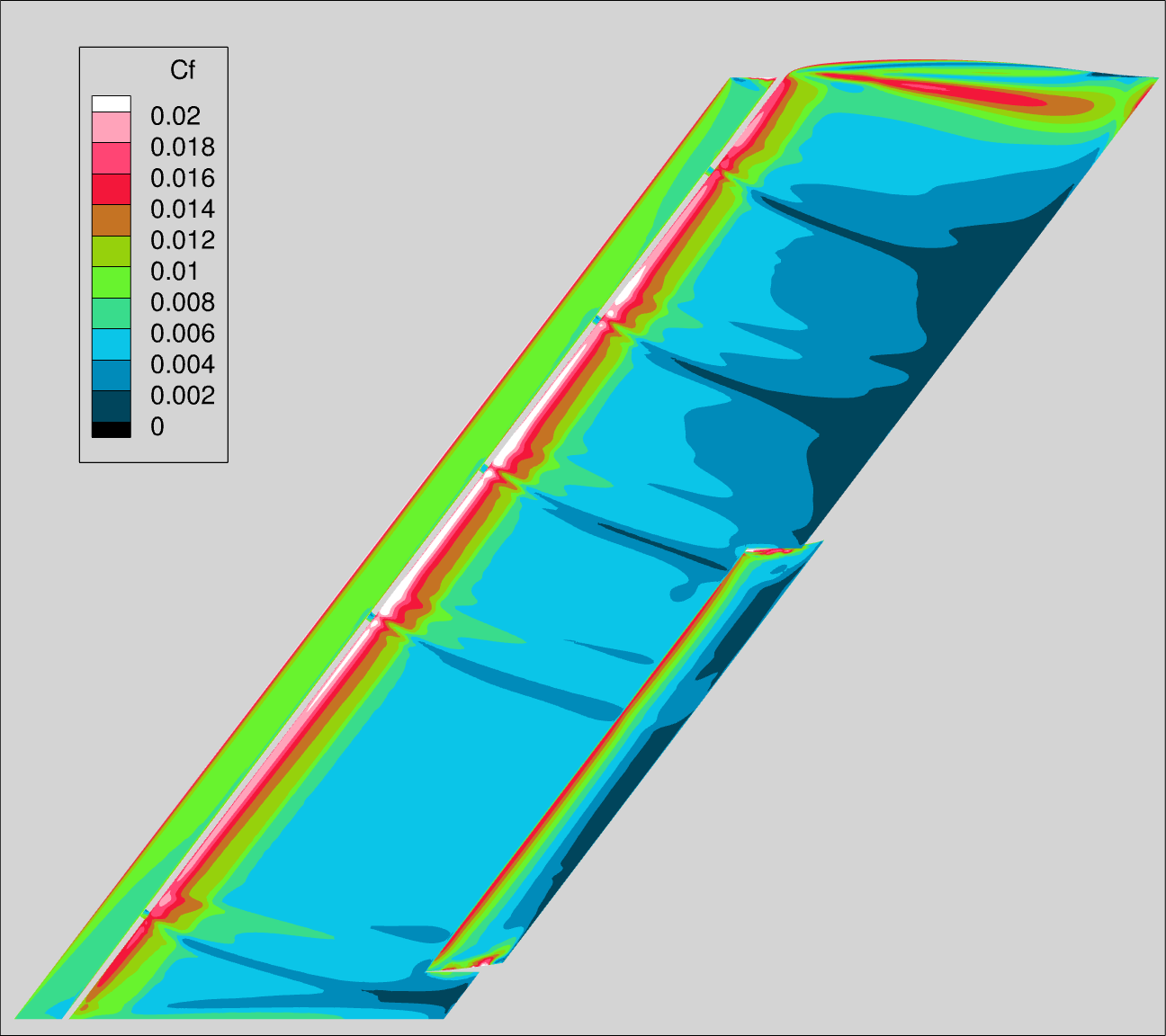
In the second figure, the Tecplot color map is provided as cfmap_tecplot.map, and the table below. The range is 0 to 0.02, step 0.002 (banded). In the Cf plots, the “lighting” should be turned off.
| LEVEL | R | G | B |
|---|---|---|---|
| 0.00 | 0 | 0 | 0 |
| 0.25 | 0 | 191 | 255 |
| 0.50 | 127 | 255 | 0 |
| 0.75 | 255 | 0 | 64 |
| 1.00 | 255 | 255 | 255 |
For direct CFD comparisons, five required views are shown below. In Tecplot, the “use perspective” feature is not turned on for any views.
A single Tecplot Layout file is included, which captures the views, the colormap settings, and streamlines. The different views are accessible through the pages feature of Tecplot. Note that Streamtraces should be enabled for the streamlines image, but disabled for the Skin Friction image.
The views are captured in the .lay file, but If additional definition is needed please reach out to your TFG leads.
VIEW_1_WING
VIEW_2_SLAT
VIEW_3_FLAP
VIEW_4_B2_TOP (Bracket #2, Top)
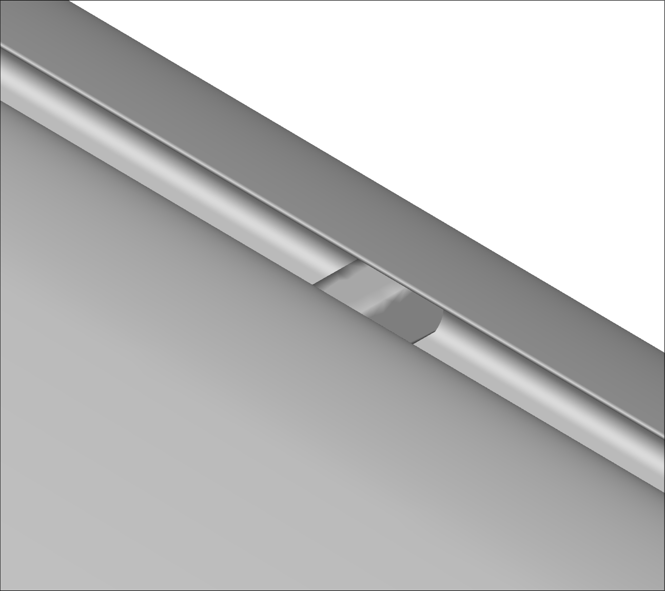
VIEW_5_B2_BOT (Bracket #2, Top)

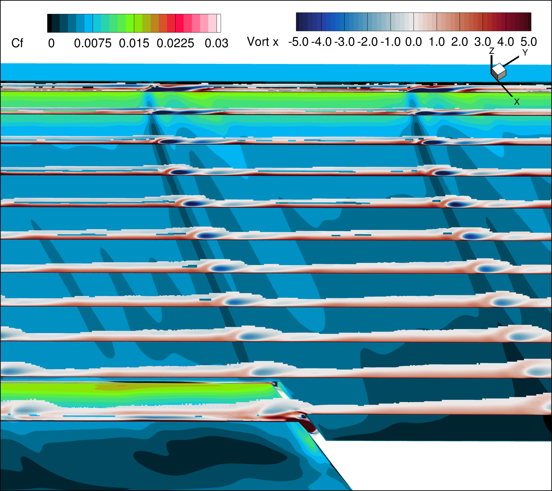
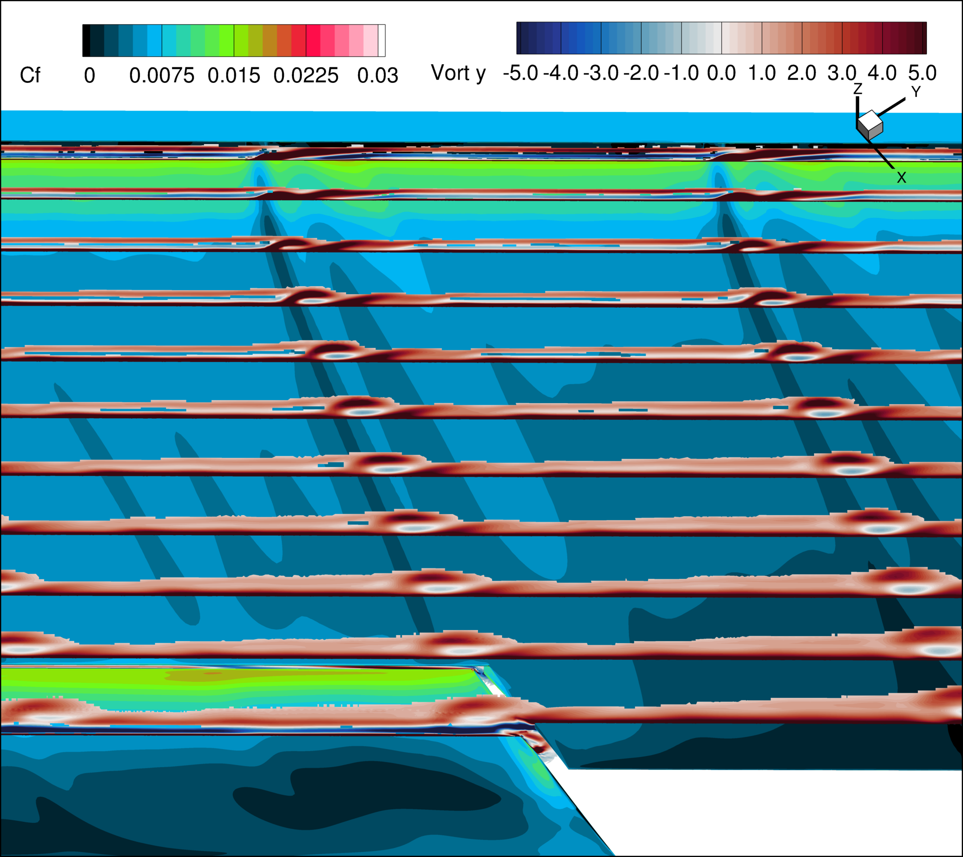
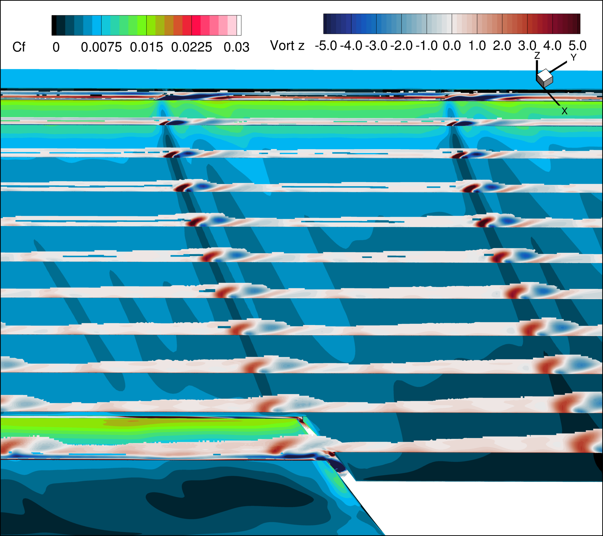
Views 6a-c visualize the wake of the slat brackets. Views 6a, 6b, and 6c display the x, y, and z components of the vorticity vector, respectively. Surface skin-friction coefficient contours are also shown on the wing. The vorticity vector within the cut planes can be provided directly by the CFD solver or processed within Tecplot.
A set of Tecplot macros is available for download. These macros define the views, volume cuts, and output variables (such as the skin-friction coefficient on the wing and vorticity on the volume cuts). Each view combines 11 cut planes; for reference, these volume cut planes are defined in 140_XXX_aoaYYY_q_view03-03.slice1.mcr within the package. To generate the views, follow these steps:
- Load the surface boundary and volume data into Tecplot, ensuring the grid system is in inches.
- Nondimensionalize the vorticity components (named “Vort x”, “Vort y”, and “Vort z”) and the vorticity magnitude (named “Vort mag”) by multiplying them by the ratio MAC/a, where MAC is the mean aerodynamic chord and a is the freestream speed of sound.
- Ensure that the skin-friction coefficient variable is named “Cf”.
- Run the main Tecplot macro, 000_all.mcr, from the downloaded package.
This macro is expected to generate three PNG files in your run directory (sample figures are shown below for an angle of attack of 10 degrees). Note that to make all cut planes visible, the nondimensional vorticity magnitude is blanked for values of 0.5 or less. For scale-resolving simulations, it is recommended to output the vorticity components and magnitude for the time-averaged flow.
Here is additional information about the setup: set a non-perspective (orthographic) camera with a 30-unit wide field; position the view at coordinates (X: 22338.8, Y: -16757.7, Z: 42984); and set the PSIAngle (about x-axis) and ThetaAngle (about z-axis) to 33 and -53 degrees, respectively. Each cutting plane is defined by the uniform normal vector [0.796715, -0.604356, 0.0] and the following origin points (all coordinates are in inches):
- Plane 1 X = 33.60, Y = 41.8497, Z = 5.5123
- Plane 2: X = 36.24, Y = 41.8497, Z = 5.5123
- Plane 3: X = 38.88, Y = 41.8497, Z = 5.5123
- Plane 4: X = 41.52, Y = 41.8497, Z = 5.5123
- Plane 5: X = 44.16, Y = 41.8497, Z = 5.5123
- Plane 6: X = 46.80, Y = 41.8497, Z = 5.5123
- Plane 7: X = 49.44, Y = 41.8497, Z = 5.5123
- Plane 8: X = 52.08, Y = 41.8497, Z = 5.5123
- Plane 9: X = 54.72, Y = 41.8497, Z = 5.5123
- Plane 10: X = 57.36, Y = 41.8497, Z = 5.5123
- Plane 11: X = 60.00, Y = 41.8497, Z = 5.5123
VIEW_6a/b/c_SLAT_BRACKET_WAKES
Postprocessing: Mean Surface Pressures and Skin Friction Extraction
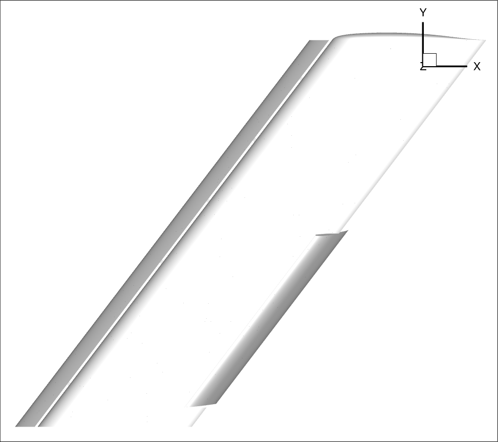
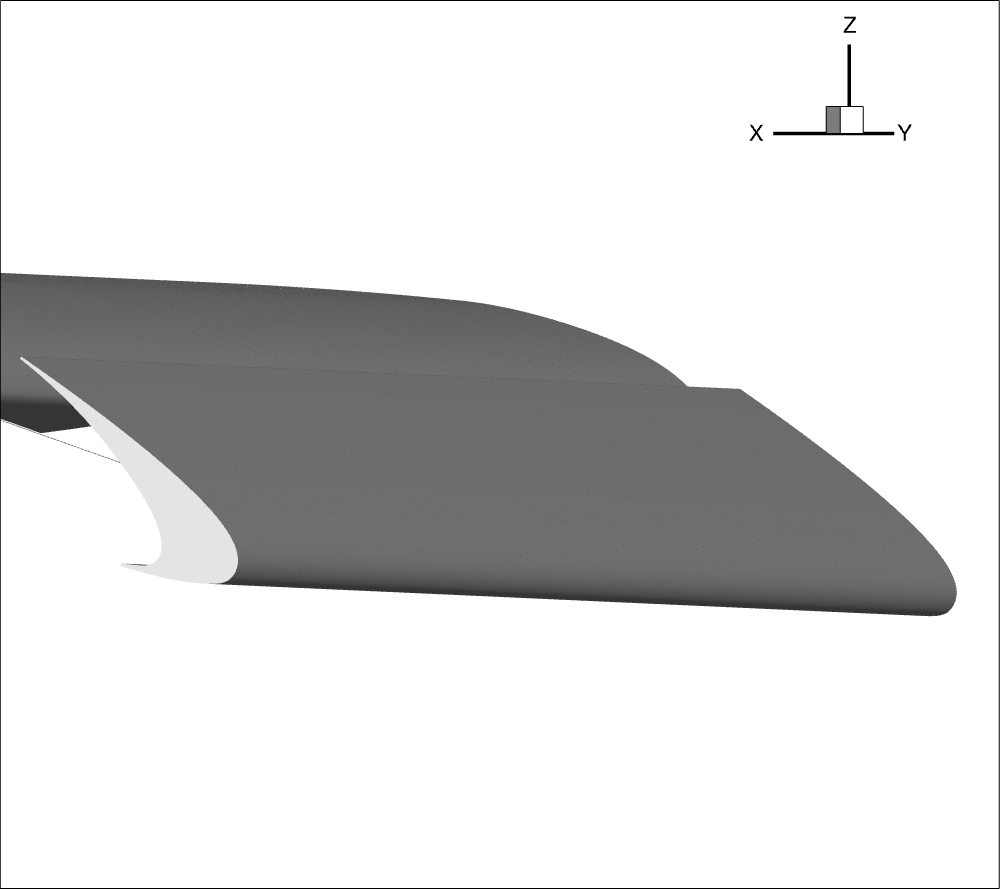
The surface data are to be extracted along several pressure rows, which are defined using the equation Ax + By + C = D. The definitions of these planes are contained in this spreadsheet, and shown graphically below.
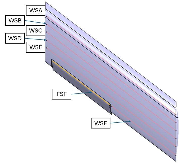
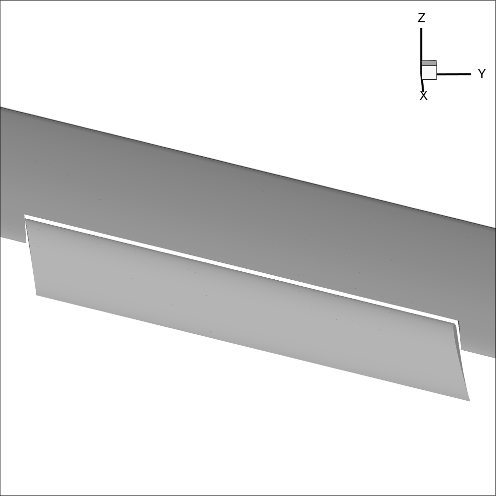
The first figure shows the basic layout of the chordwise rows. On the wing and slat, there are 7 pressure rows defined, WA through WG, and SA through SG. Each pressure row is defined by a single plane. Note that, when deployed, the pressure tap rows on the slat are not aligned with the wing (they are aligned only when stowed). The deployed flaps have 3 rows defined, FA through FC.
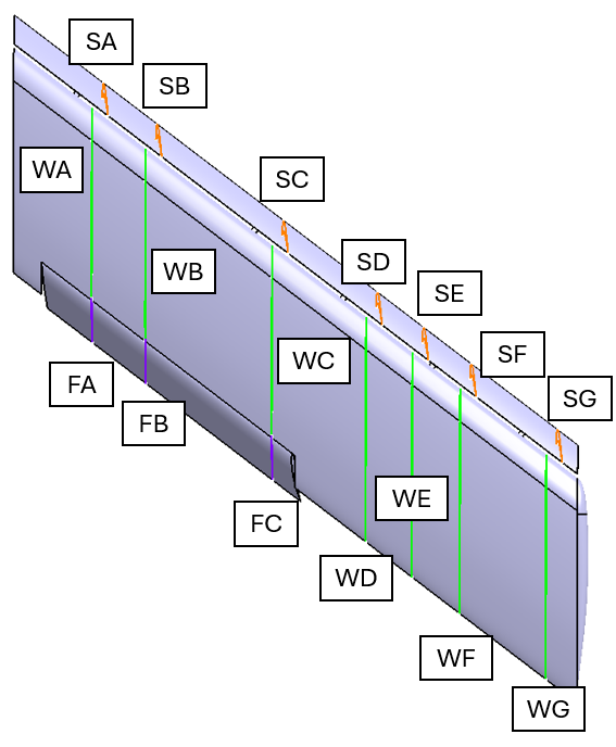
Additionally, there are 6 spanwise pressure rows defined over the wing, WSA through WSF. Note that Spanwise Row F also extends across the flap element, as belt FSF. This layout is shown in the figure below. For the spanwise rows, only data on the upper surfaces is requested though cuts through the entire upper and lower wing surface are also acceptable.